TiKZ Introductory Guide
Author: Ernesto Martínez GarcíaTags: 0013 latex tikz
Welcome to this introductory guide to the hard and horrible world of figures in LaTeX. Today we will be learning TiKZ. I personally use Typst+CeTZ for my personal work, but I recently started a PhD in Information Security, and for collaboration and publishing purposes I’m tied to LaTeX. So, I decided to learn TiKZ from the basics and stop copy pasting, hopefully.
First, let me reference two important resources:
- TiKZ Manual: https://tikz.dev/
- LaTeX Unofficial Reference: https://tug.org/texinfohtml/latex2e.html
Basic environment
Let’s start with how you can start writing a TiKZ figure:
| |
Now you can compile it with your favorite LaTeX wrapper, hoping it fixes decade-old problems inherent from LaTeX. You can also go and make a coffee in the meantime.
Another way to start a TiKZ drawing environment is inlining it:
| |
which produces:
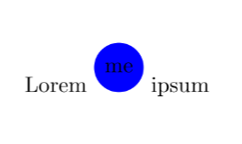
What the things inside the TiKZ environment mean will come later.
Just know that you can have a tikzpicture but also inline \tikz.
Paths, draws, fills, and nodes
Let’s study what we can write inside a tikz figure.
\path\node
The path defines, well, a path:
| |

You will see that we have not printed anything, there’s no output. That’s because we just defined a path. We just defined a path with a set of coordinates (which we will explain later), but nothing to draw on.
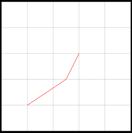
We can instruct TiKZ to please draw the path with \path[draw]:
| |
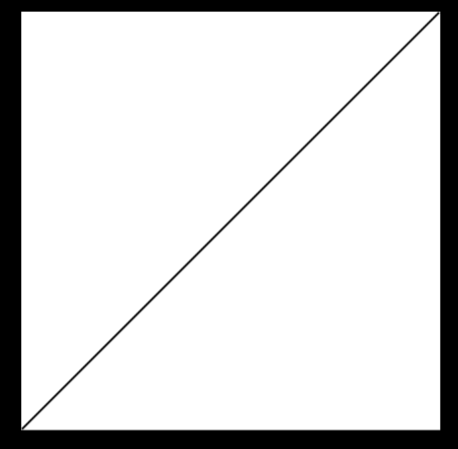
And now we get our path drawn.
\path[draw] is so used that it can be simplified as \draw! But that’s just
an abbreviation, in reality, you are writing a path.
You can also do \path[fill] to fill it with contents instead of drawing the
path, let’s see how it works:
| |
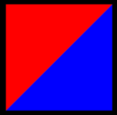
Now we were able to fill the inside contents of our path with \path[fill].
This is so used that it can be abbreviated as \draw, but that’s still a path!
Another fundamental instruction in TikZ is \node. This one is actually
different than a path. Nodes are not paths, are not part of the path either.
Rather, they are added to the picture before or after a path has been drawn.
Let’s see it with an example:
| |
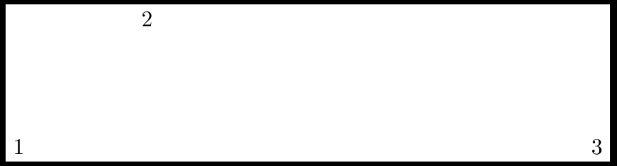
See? We placed some content (in our case, numbers) in the TiKZ figure, and these are nodes.
A very useful feature is that we can name our nodes:
| |
Nothing changes in the picture, but now we can reference this coordinates with a path or other functions:
| |
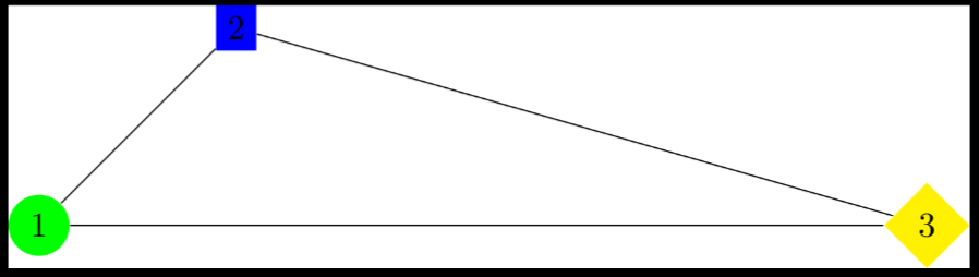
Nodes are usually shapes (a circle, a rectangle, etc). Nodes can take their
shape with the shape= argument. There are three predefined shapes by default,
but more can be added with the shapes.multipart tikz library.
- rectangle
- circle
- coordinate
Adding the shapes.XXX library via \usetikzlibrary{shapes.XXX} gives many
more shapes, see https://tikz.dev/library-shapes.
geometrictriangleellipse- …
Let’s put it to use:
| |
As shapes are very common in nodes, they have some syntactic sugar, if TiKZ doesn’t understand an option passed, it will try to understand it as a shape, thus the following is valid TiKZ and equivalent to the previous snippet:
| |
Nodes and paths can be mixed, see the following example:
| |
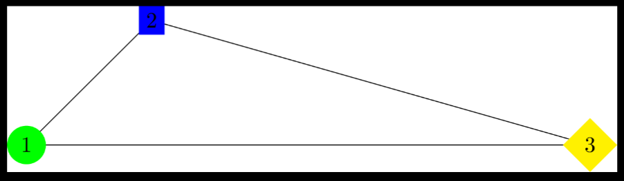
For drawing big figures not mixing paths and nodes might be better for readability, but maybe this is helpful for inline TikZ.
Coordinates
Probably not a mistery for anyone using TiKZ that coordinates exist. We have been using them previously here. But let’s give a proper explanation.
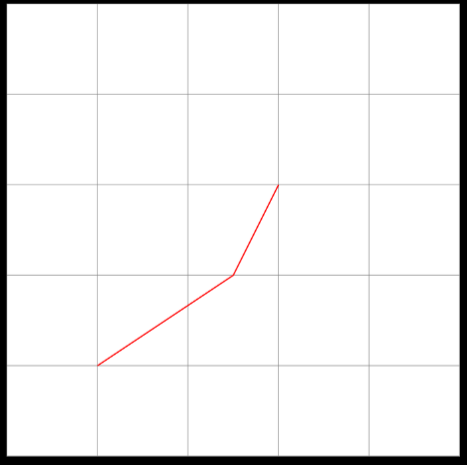
Coordinates are used to specify positions inside the TiKZ canvas, see:
| |
and changing the coordinate reflects a change in our line:
| |
There’s two ways of specifying the coordinates:
- Explicity
- Implicity
In explicit coordinates, we have to specify the coordinate system used (more on that later). In implicit coordinates, TiKZ (commonly) guesses which one you are using.
There are multiple coordinate systems:
canvasxyzcanvas polarxyz polarbarycentricnodetangentperpendicular- and your own
From all this ones, the most important for us will probably be canvas, xyz
and node. Maybe * polar if you are smart enough (I’m not).
You can, per coordinate, specify the coordinate system used (this will be an explicit specification!):
| |
See how we used the canvas coordinate system in the first coordinate
explicity, but the others don’t have it? Well, we are mixing explicit and
implicit coordinate specifications. TiKZ is guessing the coordinate system of
the last two points to be canvas.
Note: canvas cs:x=1cm,y=1cm reads as “canvas coordinate system”, and then the
specification. Might be helpful to remember the syntax.
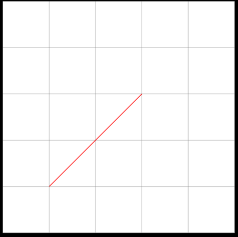
Let’s try the xyz coordinate system:
| |
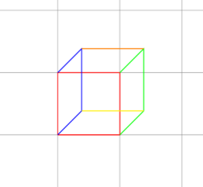
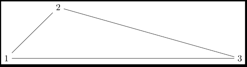
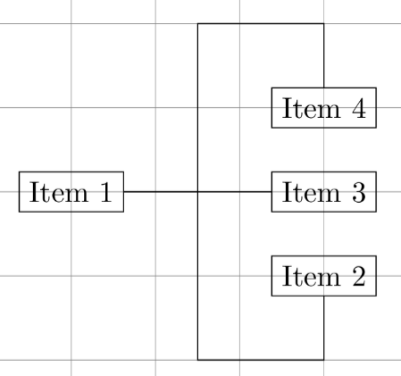
Now let’s move to the node coordinate system, which we already used in the past.
| |
See how we define 4 nodes: A, B, C, D. Then, we reference these nodes as if
there were coordinates, that’s called the node coordinate system. We draw lines
from A to C, from B to a coordinate and then A, and from D to a coordinate and
then A.
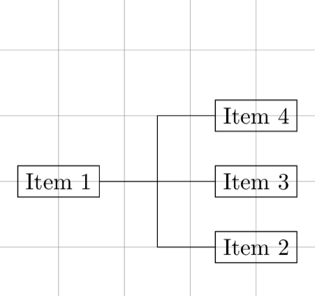
One very important note from here is the anchor option. This represents where
the path is being started from in the node.
| |
See how the anchoring defines the start of the path from the node:
TODO angles
Not providing an anchor= or an angle= means that TiKZ will calculate the
appropiate position automatically.
TODO unfinished! Will be posting more